Aperture Load Balancers
The family of aperture load balancers are characterized by their selection of a subset of backend hosts with which to direct traffic to. This stands in contrast to P2C which establishes connections to all available backends. In Finagle, there are two aperture load balancers, random aperture and deterministic aperture which differ in how they select the subset of hosts. Both of these balancers can behave as weighted apertures, which have knowledge of endpoint weights and route traffic accordingly without requiring preprocessing.
Eager Connections
Aperture Load Balancers also have a special feature called “eager connections”. What this means is that they open connections to the remote peers in their aperture eagerly. This can save time when a service is starting up, so that its persistent connections can get going quickly and the initial requests don’t need to wait for TCP connection establishment. Eager connections can be enabled or disabled service-wide with the flag com.twitter.finagle.loadbalancer.exp.apertureEagerConnections. That flag can be set to one of three values, Enabled, Disabled, and ForceWithDefault (case doesn’t matter).
Enabled turns on eager connections for the cluster that the client is configured to talk to.
Disabled disables eager connections always.
ForceWithDefault turns on eager connections for the cluster that the client is configured to talk to, as well as other clusters that the client finds itself routing to for name rewrites via dtabs. This can be useful when a service sees a small number of well-known dtabs, but can be risky if a service expects many dtabs and can risk creating too many connections.
Random Aperture
The Random Aperture load balancer was developed to reduce the number of connections that clients will establish when talking to large clusters. It does so by selecting a random subset of backends to talk do under normal conditions with some slight changes under extraordinary conditions. This a positive effect for both clients and servers by reducing the connections between them but comes with the cost of load banding. Because clients choose which servers they talk randomly, it’s possible that some choices of the minimum number of peers to talk to will cause some servers to have more clients than others. Assuming that clients in a cluster produce the same amount of load, this means that some servers will have more or less load than others. This makes it harder to reason about a clusters overall capacity, overload scenarios, and failure modes because servers are no longer uniformly loaded.
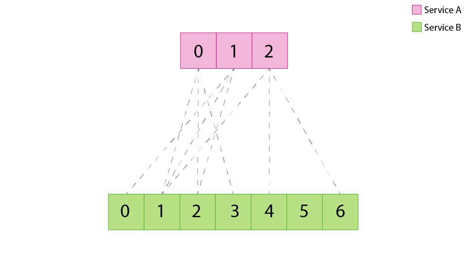
Service A connecting to Service B using random aperture. The number of connections are reduced but there is an uneven number of connections per service B host due to the statistical nature of service A picking hosts randomly.
Minimizing Banding in Random Aperture
The random aperture load distribution can be very closely approximated by the binomial distribution. The distribution represents the likelihood that a server will have a given number of clients, where a client represents a uniform amount of load. A binomial distribution can be characterized by two parameters, n and p, where n is the number of edges (trials) between the clients and the servers, and p is the probability that a given server is chosen when a client chooses an edge. In a client/server relationship,
n = (# client) * (# remote peers per client)
p = 1 / (# servers)
The distribution can be used as a guide for how to choose the number of remote peers per client. Since the binomial distribution starts to turn Gaussian as the increase the number of trials, properties of Gaussian distributions can be used to reason about the binomial distribution (note that it’s worth checking that the graph looks reasonably Gaussian before using these rules of thumb). In a Gaussian distribution, approximately 1/3 of the servers will be < (mean - stddev), and approximately 1/3 of the servers will be > (mean + stddev). This can be used to extrapolate the distribution of connections per host. Wolfram Alpha is a good resource for visualizing the behavior of a binomial distribution for different parameters.
Example
Let’s say that there exists a service called “Brooklyn” that has 1000 nodes in its cluster which is configured to use the aperture load balancer to connect with a service consisting of 5000 nodes called “GadgetDuck”. The goal is to pick the minimum number of connections that will result in a ~20% or less difference between the low and high load bands. As an initial value for exploring the distributions, the asymptotic value of 1 is used as the aperture size. Using Wolfram Alpha, the mean is found to be 5, and the stddev will be 2.5. This distribution is too wide to satisfy the 20% difference requirement, so the next step is to increase the number of remote peers to 10. Wolfram Alpha computes the mean and stdev of the new distribution to be 50 and 7, respectively, which is still too wide. A third attempt using 100 remote peers yields a mean of 500 and stddev of 22 which is within the requirements. Thus, an aperture size of 100 or more will satisfy the load banding requirement. Further iterations could be used to shrink the aperture size to a value in the range (10, 100] that still satisfies the banding requirement, if so desired.
Deterministic Aperture
Deterministic aperture is a refinement of random aperture that has better load distribution and connection count properties. Like random aperture, deterministic aperture reduces the overhead of clients for both clients and the servers they talk to by only talking to a subset of service instances, unlike P2C which lets the client pick from any replica in the serverset. However, unlike the classic aperture implementation, it does so using a deterministic algorithm which distributes load evenly across service instances, reducing the phenomena of load banding which is inherent to the statistical approach employed by random aperture. This facilitates a further reduction in necessary connections and manual configuration. Deterministic Aperture is the default load balancer at Twitter.
Service B RPS during a rolling restart of service A which changed the load balancer from random aperture to determinstic aperture
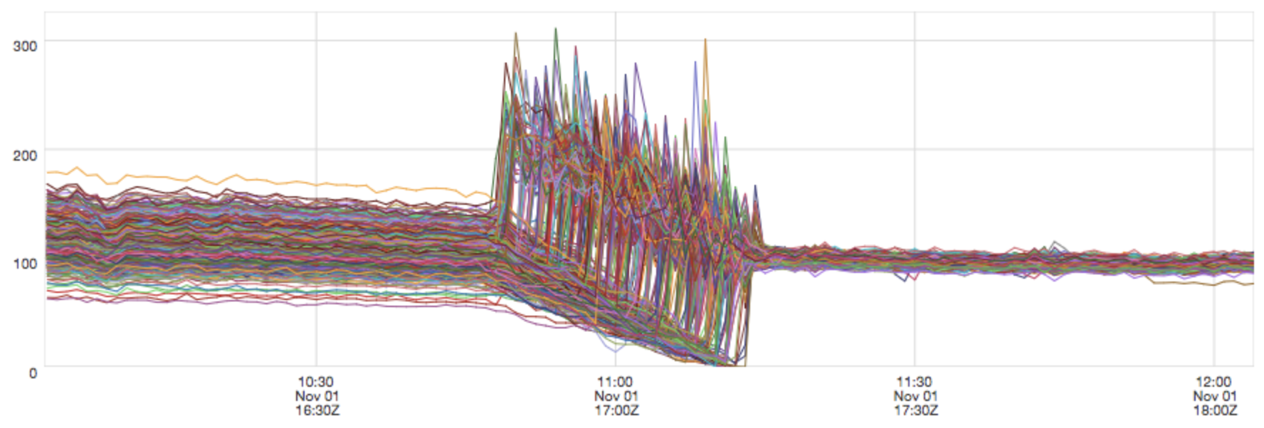
The variance in requests per second (RPS) is significantly diminished after the service A deploy due to the deterministic load distribution.
Connections from service A to service B during a rolling restart of service A which changed the load balancer from random aperture to determinstic aperture
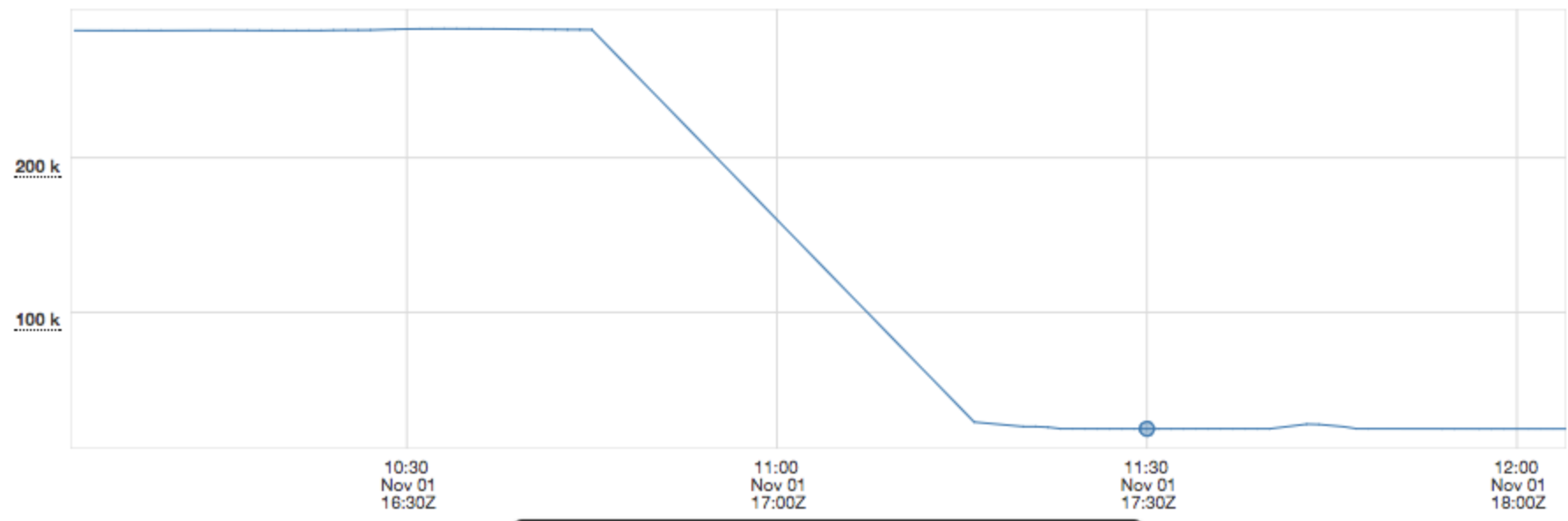
The total number of connections from A to B was significantly reduced.
Deterministic Subsetting
Deterministic aperture combines information about both the backend cluster as well as the cluster information for the service at hand and partitions connections to backends in a way that favors equal load and minimal connections (with a lower bound of 12 to satisfy common concurrency and redundancy needs). It does this by letting each member of a cluster compute a subset of weighted backends to talk to based on information about each cluster. This can be visually represented as a pair of overlapping rings: The outer ring, or “peer ring”, represents the cluster of peers (Service A) which are acting in concert to offer load to the “destination ring” which represents the cluster of backends (Service B).
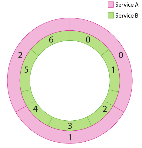
Each instance of Service A determines which “slice” of the backend ring to talk to and directs its traffic to those specific instances.
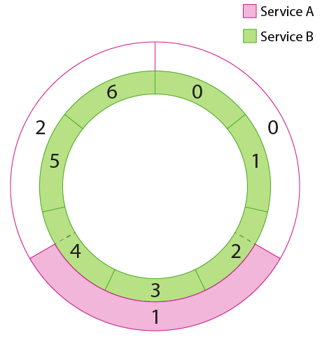
Since each client instance is doing the same thing, except picking the slice that belongs to them, we can evenly load the backend cluster (Service B). Note that this requires the load balancer to respect the continuous ring representation since peer slices may cover fractional portions of the destination ring.
Traffic Patterns
The deterministic aperture model, and subsetting models in general, works well when the traffic pattern between service A and B is “smooth” meaning that for each instance of Service A the request pattern doesn’t consists of significant bursts with respect to the average request rate and that requests are roughly equal cost, both in resource usage of the backend and in terms of latency. If the traffic pattern is characterized by large bursts of traffic, say invalidation of a cache based on a timer, then small chunks of the ring will end up extremely loaded for the duration of the burst while other slices may be essentially idle. Under those conditions the P2C load balancer may be more appropriate so the entire backend cluster can absorb the large bursts coming from instances of Service A.
Peer Information
In order for deterministic aperture to be deterministic it needs to know some additional information. This is important for computing the “slice” of backends that the load balancer will utilize. To know how large of slice to use the client needs information about both the backends, or the serverset, and it needs to know some information about its peers, also known as the peerset. The peerset is the only new information needed since knowing about the backends is a requirement for any client side load balancer. In regard to the peerset we need two different pieces of information:
How many replicas are there in the peerset. This is used to compute how large each clients slice of the backends will be.
What is the position of this instance in the peerset. This is required to compute which slice that this client should take.
This information can be configured in the ProcessCoordinate object by setting the processes instance number and the total number of instances. The current implementation requires that all instances in the cluster have unique and contiguous instance id’s starting at 0.
Key Metrics
Success rates and exceptions should not be affected by the new load balancer. Other important metrics to consider are request latency and connection count.
$clientName/request_latency_ms.p*

$clientName/connections

$clientName/loadbalancer/vector_hash

finagle/aperture/coordinate
Weighted Aperture
The weighted “flavor” of aperture load balancers was introduced as a means to offer balancers more control over balancing traffic. Traditional aperture balancers require preprocessing to generate groups of equally weighted endpoints, allowing the load balancer to send the same proportion of traffic to each endpoint. Weighted aperture balancers, on the other hand, need no pre-processing. They have knowledge of endpoint weights and send traffic proportionally. Apart from allowing these balancers to behave more dynamically, this limits the number of connections going to any single instance. For example, an endpoint with a unique weight, no matter how small, would, in traditional balancers, end up in its own weight class alone, therefore appearing in every aperture and receiving many connections. With weighted aperture, that endpoint would simply occupy a smaller portion of the ring and therefore appear in fewer apertures. Though both Random and Deterministic Aperture can behave as weighted aperture balancers, their algorithms are slightly modified to account for this additional information.
Weighted Deterministic Aperture
With additional weight information, the ring model is no longer a simple abstraction for selecting endpoints to send traffic to. If endpoints can handle differing levels of traffic, they can’t take up equal portions of the ring. In other words, the “fair die” feature of the ring is abandoned. The ring in the examples above might look something like the following.
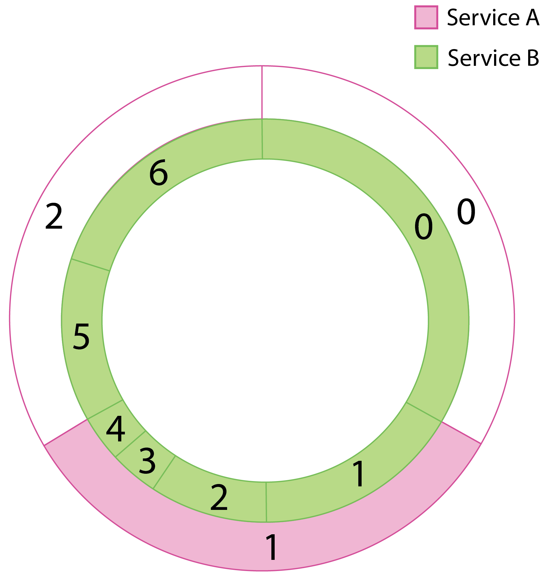
Without some computation, it’s not immediately obvious which endpoints are within the aperture, nor is it easy to determine which endpoint a value between 0 and 1 corresponds to, making random selection within an aperture equally difficult.
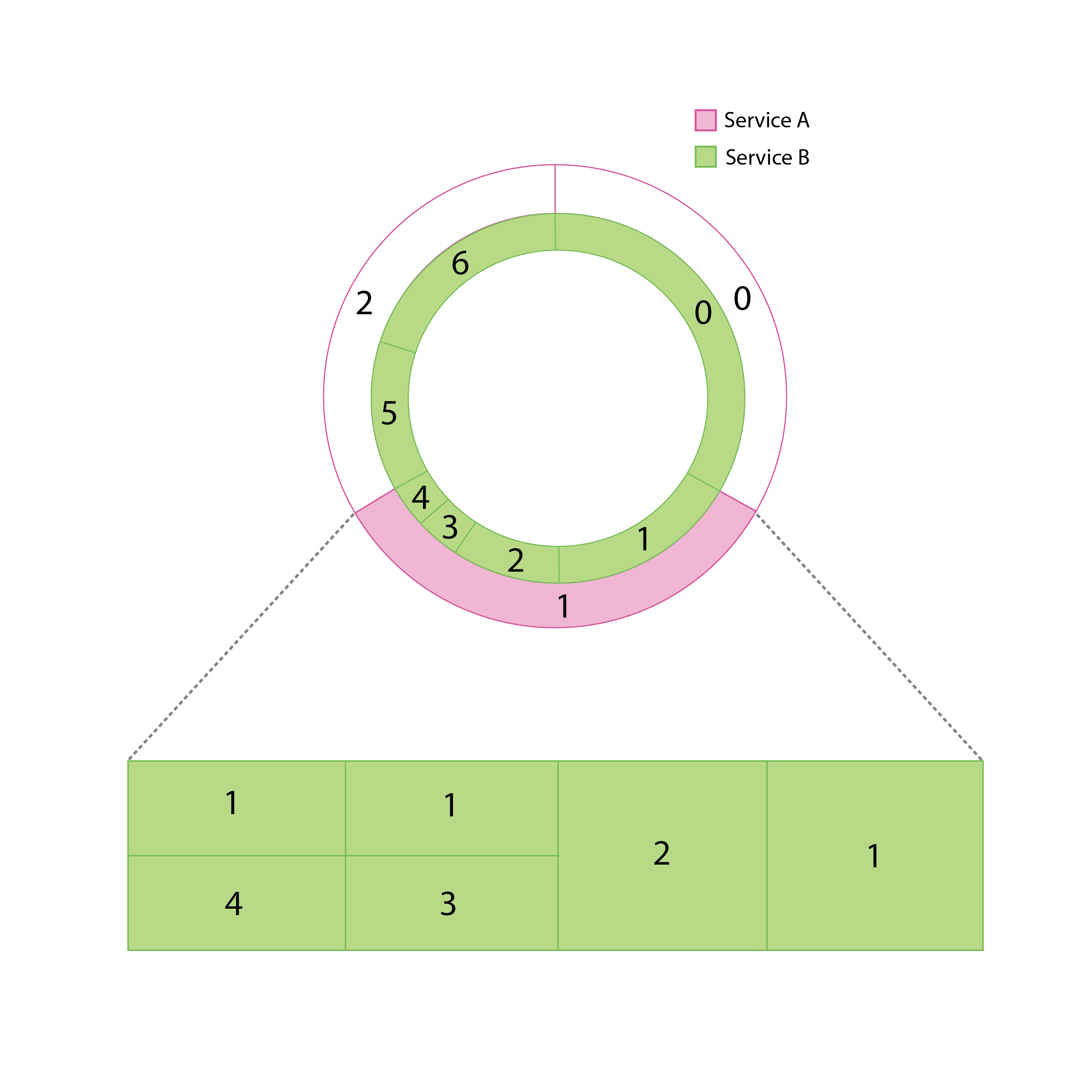
Rather than representing the deterministic subsetting for weighted aperture as overlapping rings, we shift to a two dimensional model that represent the nodes within a given aperture as reorganized areas.
Mathematically, this computation is completed via c.t.f.util.Drv. By adding a second dimension, we’re able to equalize the widths of each endpoint while maintaining their weights in the form of areas. For example, an endpoint of weight 0.5 would, rather than having a length around a ring of 0.5, have a width of 1 and a height of 0.5, resulting in an overall area of 0.5. Crucially, this reorganization retains the O(1) complexity of the original ring model by making indexing simple.
For more information on how determinism is maintained in weighted aperture balancers, check out c.t.f.util.Drv and this explanation of the probabilistic models.
Weighted Random Aperture
Similarly for random aperture, the problem of identifying endpoints when they’re each of different widths (or lengths) isn’t as simple in the weighted pathway. As an added complexity, endpoints in random apertures are occasionally reorganized to ensure healthy nodes are more often within a given aperture. Since building the Drv is costly, rebuilding it at unknown intervals is unreasonable. Therefore, for weighted random aperture, we still arrange the endpoints along a ring bounded betweeen 0 and 1 but instead use binary search to determine which endpoint is selected by P2C. It’s important to note that this change results in a shift from O(1) endpoint selection to O(log(N)) selection complexity. This is a compromise made to ensure that the overall behavior of Random Aperture is maintained.
Key Metrics
The key metrics for weighted apertures are the same as their traditional counterparts, with one exception. To determine if you’re running a weighted balancer, check for the _weighted suffix in the $clientName/loadbalancer/algorithm metric.